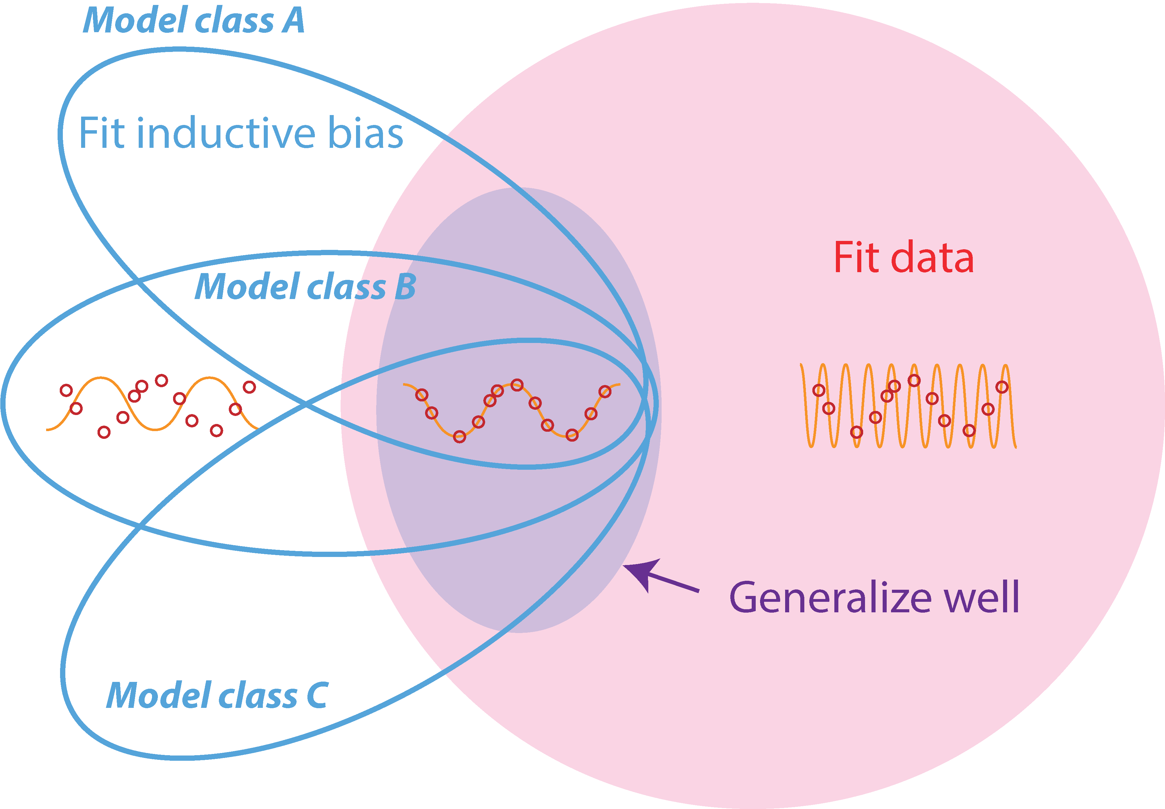
Figure 1: An illustration of the hypothesis space of a task. Hypotheses may or may not fit the training data (red region) or contain particular sets of inductive biases; different blue ovals correspond to different model classes (i.e. different sets of inductive biases). Together with training data, specific choices of model class can restrict hypotheses to a well-generalizing region; purple indicates well-generalizing hypotheses. Both training data and inductive biases are required to generalize well.

Welcome to our blog post on measuring generalization difficulty in machine learning! In this post, we will introduce our paper that presents a model-agnostic measure of generalization difficulty. This measure allows us to quantify the inherent challenges faced by machine learning algorithms when it comes to generalizing well on different tasks.

What Is Inductive Bias and Why Is Measuring It Important?

In the field of machine learning, researchers have long recognized the importance of inductive bias in achieving successful generalization. Inductive bias refers to the constraints or assumptions that a model designer incorporates into a machine learning model, enabling it to generalize from limited training data to unseen test data. For instance, convolutional neural networks (CNNs) are designed to exploit the spatial structure of images, while recurrent neural networks (RNNs) are designed to exploit the temporal structure of sequences. These inductive biases allow CNNs and RNNs to generalize well on image and sequence data, respectively.

Thus, inductive bias can be thought of as the set of assumptions or constraints that a model designer imposes on a machine learning model. Tasks requiring greater inductive biases require more effort from a model designer to achieve successful generalization: they are more difficult from the model designer’s perspective.

However, despite the central role of the concept of inductive bias in machine learning, the quantification of inductive bias has remained a challenge in general learning settings. One of the key implications of quantifying inductive bias is its potential to guide the design of more challenging tasks. By increasing the complexity of the inductive biases required for successful generalization, we can push the boundaries of machine learning and promote the development of stronger models and architectures.

In this paper, we present a novel information-theoretic framework that allows us to systematically evaluate the inductive bias complexity of various tasks across different domains, including supervised learning, reinforcement learning, and few-shot meta-learning.

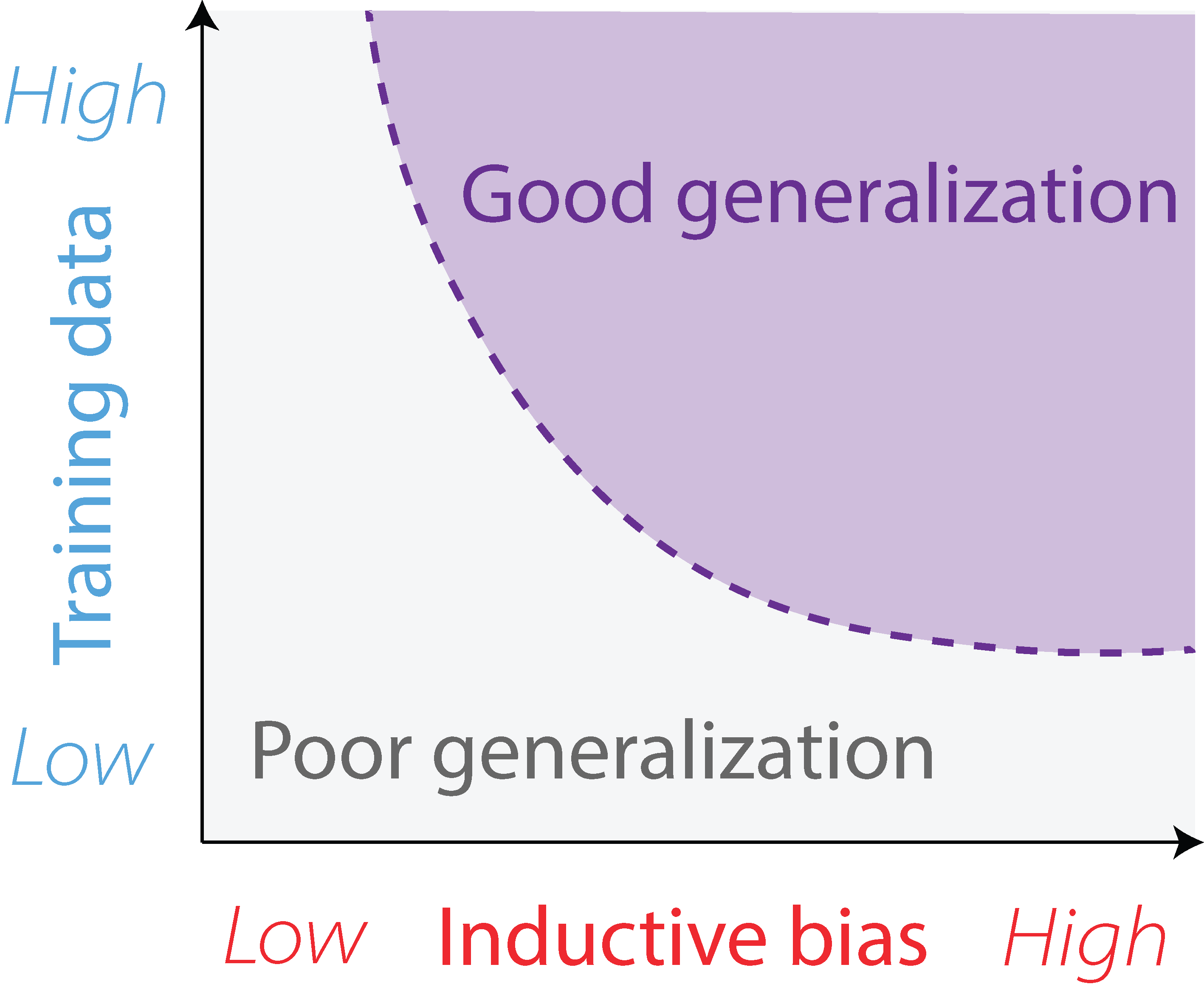
Figure 2: Tradeoff between sample complexity and inductive bias complexity. Tasks with higher inductive bias complexity require less training data to generalize well, while tasks with lower inductive bias complexity require more training data to generalize well.

Defining Inductive Bias Complexity

To understand inductive bias complexity, it is important to first grasp the concept of sample complexity. Sample complexity refers to the amount of training data required for a model to generalize well, given a fixed inductive bias or model class . It quantifies the minimum number of examples needed to achieve a certain level of performance.

Inductive bias complexity, on the other hand, measures the amount of inductive bias required to generalize well, given a fixed amount of training data. It focuses on the constraints or assumptions needed to guide a model’s learning process and enable it to make accurate predictions beyond the training data. Just as sample complexity is specific to a particular set of inductive biases, inductive bias complexity is specific to a particular training set. Importantly, inductive bias complexity is not a property of a model class (just as sample complexity is not a property of a training set). As Figure 2 illustrates, inductive bias complexity can be traded-off with sample complexity: a task with a higher inductive bias complexity requires less training data to generalize well, while a task with a lower inductive bias complexity requires more training data to generalize well.

To formally define inductive bias complexity, we use the notion of a hypothesis space. A hypothesis space consists of a set of possible models that could be used to solve a task. For each task, we will define a broad and general hypothesis space that includes all possible model classes that could reasonably be used to solve the task. Importantly, our notion of a hypothesis space is purely a property of the task. The hypothesis space is not the same as the model class used in practice, such as neural networks. Instead, it serves as a mathematical tool to analyze the properties of the task itself. Please see Figure 1 for an illustration of a hypothesis space.

Inductive bias complexity can then be understood as the amount of information required to specify well-generalizing hypotheses within the set of hypotheses fitting the training data. In other words, it is the minimum amount of information required to select a hypothesis that generalizes well. Formally, inductive bias complexity \(\tilde I\) is:

\[\tilde{I} = -\log \mathbb{P}(e(\theta,p)\le\varepsilon\mid e(\theta,q) \le \epsilon)\]

where \(\theta\) represents a hypothesis sampled from the hypothesis space, \(e(\theta,p)\) is its error rate on the test set, \(e(\theta,q)\) is its error rate on the training set, \(\epsilon\) is training set error, and \(\varepsilon\) is the desired test set error. This equation simply reflects the intuition that the amount of information needed to generalize is the amount of information needed to select a hypothesis that generalizes well, given that it fits the training data.

Practically Computing Inductive Bias Complexity

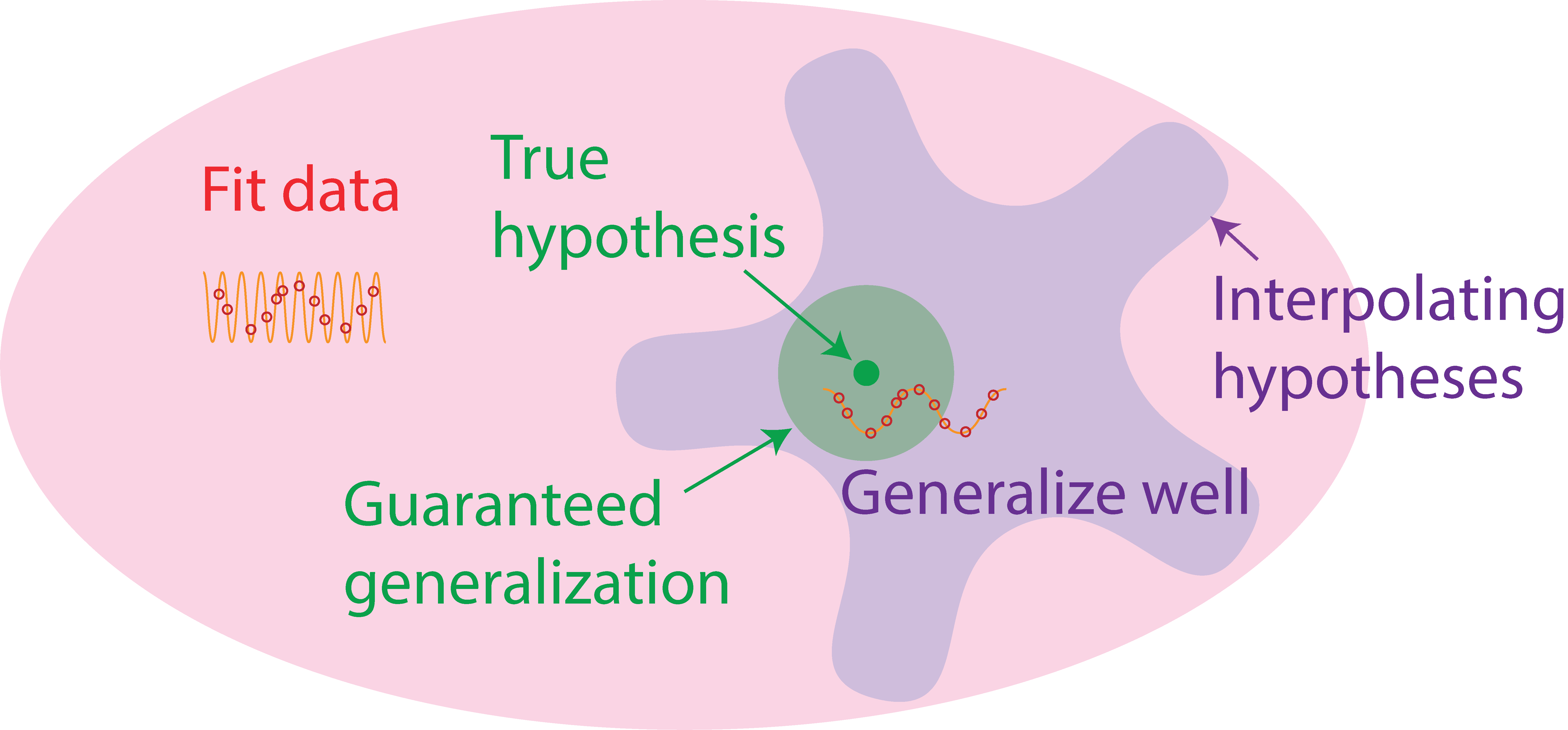
Figure 3: Illustration of the inductive bias complexity bound. Regions of the hypothesis space within a certain radius around the true hypothesis are guaranteed to generalize well. The inductive bias complexity is upper bounded by the amount of information required to specify a hypothesis within this radius.

While the above equation for inductive bias complexity provides a theoretical framework for understanding the concept, it is not always practical to compute in practice. To address this issue, we propose a series of approximations that allow us to arrive at a computable, practical measure of inductive bias complexity.

To begin, we bound the inductive bias complexity by guaranteeing generalization in a small radius around the true hypothesis, as illustrated by Figure 3. This approach allows us to more easily quantify the size of well-generalizing regions in the hypothesis space.

\[\tilde{I} \le -\log \mathbb{P}\left(d(\theta,\theta^*)\le\frac{\varepsilon}{L_\mathcal{L}L_fW(p,q)} \mid \theta\in\Theta_q\right)\]

where \(\theta^*\) is the true hypothesis, \(d(\theta,\theta^*)\) is the distance between \(\theta\) and \(\theta^*\), \(L_\mathcal{L}\) and \(L_f\) are constants, and \(W(p,q)\) is the Wasserstein distance between the training and test distributions. This equation reflects the fact that the inductive bias complexity is upper bounded by the amount of information required to specify a hypothesis within a certain radius around the true hypothesis. Intuitively, the radius shrinks as the desired test set error increases, making it harder to guarantee generalization. Similarly, as the distance between the training and test distributions increases, the radius shrinks, making it harder to generalize.

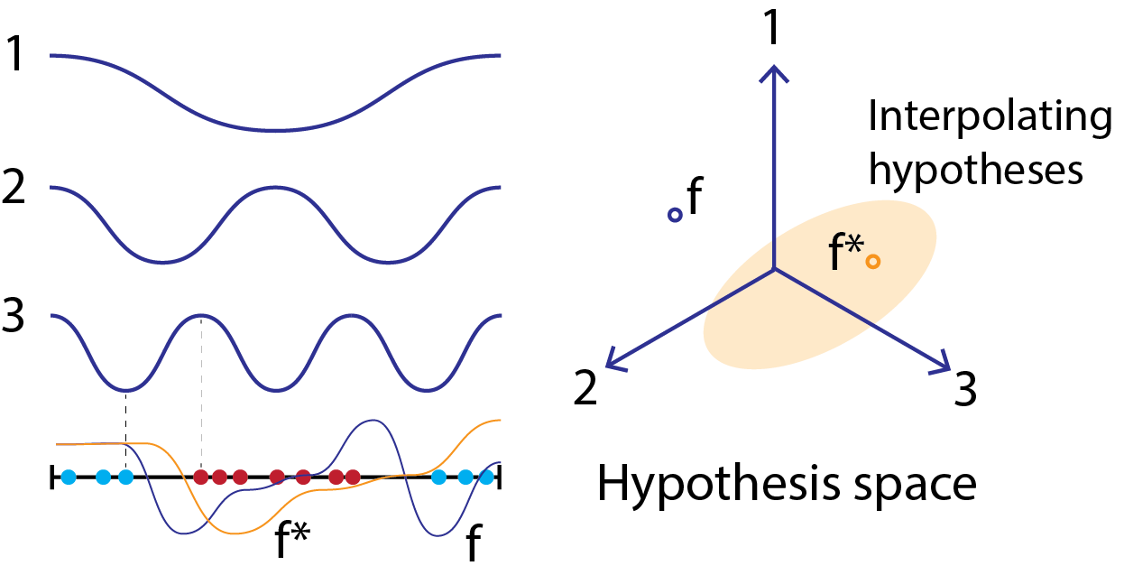
Figure 4: An example of constructing a hypothesis space for a binary-classification task with a 1 dimensional input. The black line indicates the data manifold and the blue and red dots on the line indicate training points. The hypothesis space is constructed using basis functions of three different frequencies; observe that the highest frequency is chosen to have scale corresponding to the minimum distance between classes. Two specific hypothesis are illustrated in the hypothesis space, the true hypothesis (in orange), \(f^*\) and another hypothesis \(f\) (in purple). Both can be expressed as linear combinations of the basis functions, and thus correspond to points in the hypothesis space as illustrated. The \(f^*\) hypothesis fits the training data, and thus is part of the interpolating hypothesis set indicated by the light orange oval.

In order to progress further, we must make some assumptions about the hypothesis space. We set the hypothesis space as linear combinations of eigenfunctions of the Laplace-Beltrami operator on the manifold on which the data lie. What is the Laplace-Beltrami operator? It is a differential operator that generalizes the Laplacian to curved surfaces. It is a measure of the curvature of the data manifold. The eigenfunctions of the Laplace-Beltrami operator are analogous to the Fourier basis on a flat surface. Thus, we essentially parameterize the hypothesis space as a linear combination of these Fourier-like basis functions. Importantly, we cut off the frequency of these functions: very high-frequency functions are not allowed. This is a reasonable assumption, as very high-frequency functions will not reasonably be used in practical model classes. The specific frequency cutoff is a property of each task; we set a higher cutoff for tasks requiring higher spatial resolution (i.e. more fine-grained details in the input space) to solve. Please see Figure 4 for an illustration of our hypothesis space construction.

After a series of approximations, we arrive at a practical measure of inductive bias complexity that can be computed using standard machine learning tools. We present this measure in the case of a classification task (although a similar result can be found for other settings):

\[\tilde{I} \approx (2d^2E-nd) \\ \left(\log b + \frac{3}{2}\log d + \log K - \frac{1}{m}\log n - \log\frac{\varepsilon}{L_\mathcal{L}} + \log c\right)\]

where \(d\) is the number of classes, \(n\) is the number of training data points, \(\varepsilon\) is the target error, \(L_\mathcal{L}\) and \(b\) are constants, and \(K\) and \(E\) are functions of \(m\) and the maximum frequency \(M\) of hypotheses in the hypothesis space. \(c=\sqrt{\frac{m}{6}}\left(\frac{2\pi^{(m+1)/2} d}{\Gamma\left(\frac{m+1}{2}\right)}\right)^{1/m}\), which is roughly constant for large intrinsic dimensionality \(m\) and \(E\) scales as \(M^m\).

We note some key trends from this equation: first inductive bias complexity is exponential in the intrinsic dimensionality \(m\) of the data. This is because the dimensionality of the hypothesis space scales exponentially with intrinsic dimensionality: each additional dimension of variation in the input requires hypotheses to express a new set of output values for each possible value in the new input dimension. Because inductive bias complexity is the difficulty of specifying a well-generalizing hypothesis, it scales with the dimensionality of the hypothesis space. Second, inductive bias complexity is linear in the number of training data points \(n\). Intuitively, this is because each training point provides roughly an equal amount of information about which hypotheses generalize well. Finally, note that inductive bias complexity is polynomial in the frequency cutoff \(M\) of the hypothesis space. Intuitively, this is because changing the maximum frequency allowed in hypotheses merely linearly scales the number of hypotheses along each dimension of the hypothesis space, yielding an overall polynomial effect.

Empirical Inductive Bias Complexity of Benchmarks

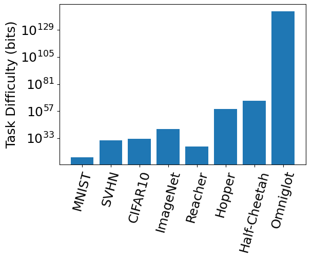
Figure 5: Inductive bias complexities (i.e. task difficulties) of various benchmark tasks across domains.

To validate our measure of inductive bias complexity, we conducted experiments on several standard benchmarks in supervised classification, meta-learning, and reinforcement learning . Our results in Figure 5 show that the inductive biases required by these benchmarks are very large, far exceeding the practical model sizes used in practice. These large numbers can be attributed to the vast size of the hypothesis space: it includes any bandlimited function on the data manifold below a certain frequency threshold. Typical function classes may already represent only a very small subspace of the hypothesis space: for instance, neural networks have biases toward compositionality and smoothness that may significantly reduce the hypothesis space, with standard initializations and optimizers further shrinking the subspace. Moreover, functions that can be practically implemented by reasonably sized programs on our computer hardware and software may themselves occupy a small fraction of the full hypothesis space. Future work may use a base hypothesis space that already includes some of these constraints, which could reduce the scale of our measured task difficulty.

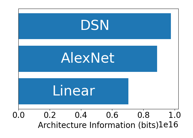
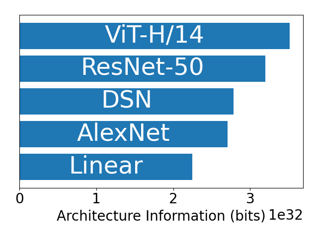
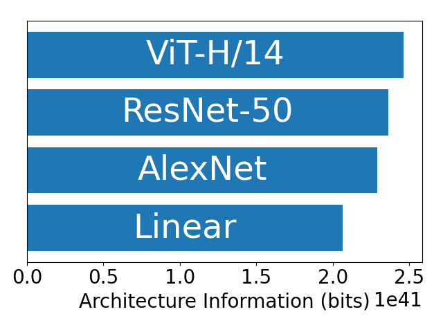
Figure 6: Inductive bias provided by different model architectures on MNIST, CIFAR-10, and ImageNet (left to right). The inductive bias complexity of a task is the minimum complexity of a model architecture that can solve the task with a desired error rate. The inductive bias of a model is measured as the required inductive bias needed to each the performance achieved by the model.

Next, we considered how much inductive bias different model architectures provide to different tasks. In Figure 6, we found that more complex tasks extract more inductive bias from a fixed architecture.

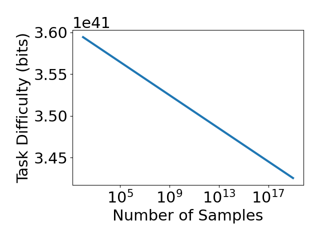
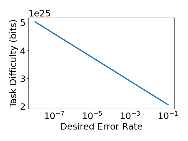
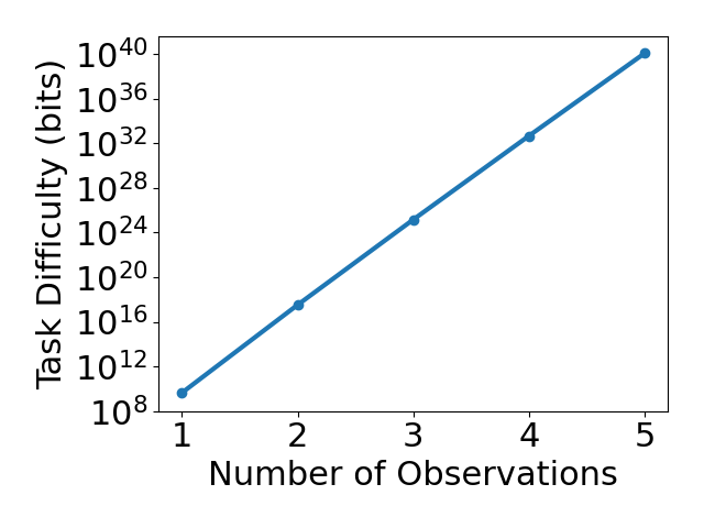
Figure 7: Inductive bias complexity of ImageNet (left), Reacher (middle), and Cartpole (right) as a function of the number of training data points, the desired error rate, and the intrinsic dimensionality of the data, respectively.

Finally, we considered how parametric variations of tasks affect inductive bias complexity. We considered the effects of varying the number of training data points, the desired error rate and the intrinsic dimensionality of the data. In Figure 7, we found that inductive bias complexity decreases quite slowly with the number of training data points and desired error rate, but increases exponentially with the intrinsic dimensionality of the data. These results are consistent with our theoretical analysis and suggest that increasing the intrinsic dimensionality of the data is a more effective way to increase the required inductive biases of a task than decreasing the number of training data points or increasing the desired error rate. One simple method of increasing intrinsic dimensionality is simply to add noise to the inputs of a task.

Conclusion

In conclusion, inductive bias complexity quantifies the information needed by a model designer to generalize effectively. It not only highlights the significant inductive biases required by standard benchmarks, but also provides a guide to task design: for instance, it suggests constructing tasks with a inputs of a high intrinsic dimensionality. We hope future work can refine our estimates and make inductive bias complexity an even more useful tool for task design and model interpretability.

Thank you for reading our blog post! If you have any questions or comments, please feel free to reach out to us.